Intro to Data Analysis
Once we got a brief introduction to both numpy and pandas, it is time to start our first Data Analysis project.
There are so many technologies out there so it might become overwhelming to expect yourself to remember all new methods and functions. The truth is: no one knows them all. Even data scientists with 900 light years of experience constantly google stuff or read docs. Our goal here is to show you, how using numpy and pandas can build a flowing narrative in data science project, so you can return to these notes any time you’ll need to refresh something.
The best definition for data analysis would be trying to answer a question using data. And it really is just this, in a nutshell. But, as it always have been, devil in the details. It’s all the specificities of the context of the field you’re working in and generally accepted approaches to solve that kind of questions in that particular field that makes data analysis so difficult to generalise - even for a definition.
Just as an illustration: all examples below are using data analysis to answer their questions, from daily tasks to space research:
- Bioinformatics 🧬: Can we identify genes that are differentially expressed in lung cancer patients compared to healthy individuals? source
- Music Taste 🎧: What songs do I listen the most? source
- Personal Time Management ⏳: Which daily habits correlate with high productivity? source
- Environmental Sciences 🌱: How can we predict earthquakes better? source
- Real Estate Market 🏡: What is the current trend in Bergen real esstate market? source
- Winter Sports Medicine ⛷️: What biomechanical factors contribute to ACL injuries in skiers? source
- Space Sciences 🌌: Can gravitational waves help reveal black holes origin? source
- Pokemons 🐭: “What are the different Pokemons types?” source
Lets meet our data
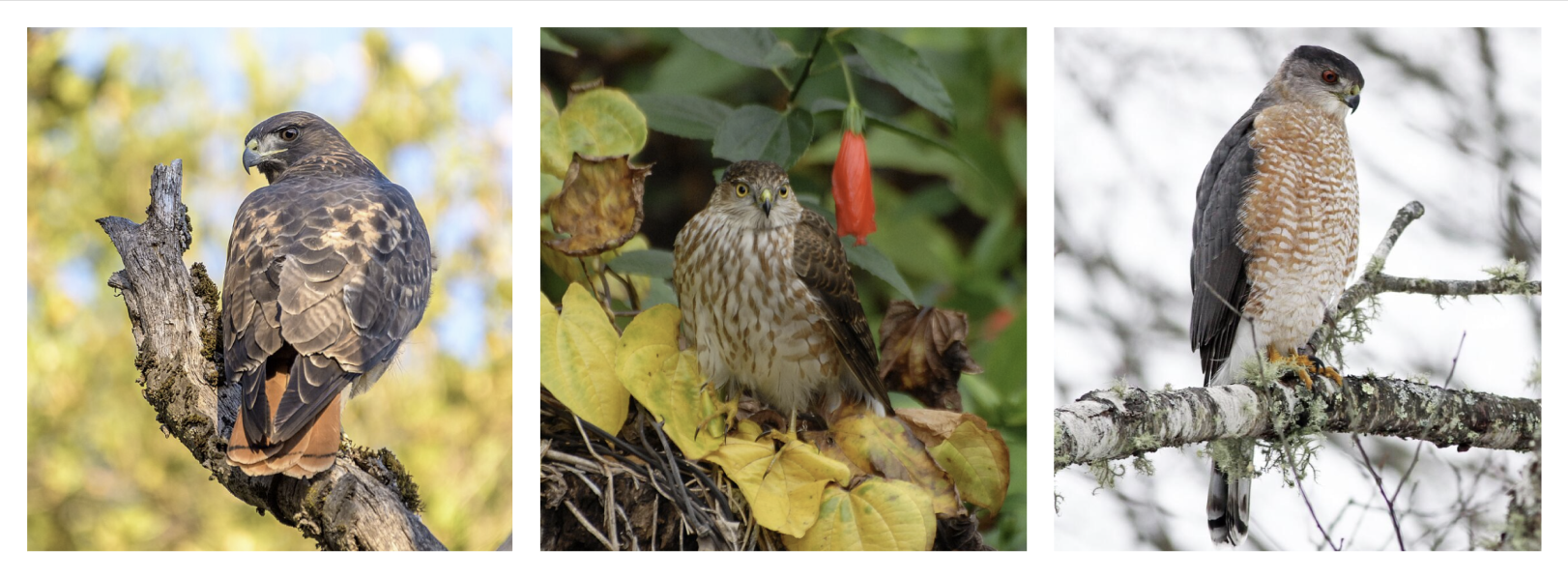
Today, we’re going to work with the dataframe about Hawks. The data was collected during bird capture sessions by students and faculty at Cornell College in Mount Vernon, Iowa, USA. The dataset include birds of the following species: Red-tailed, Sharp-shinned, and Cooper’s hawks:

(images from wikipedia and allaboutbirds.org)
import pandas as pd
import numpy as np
hawks = pd.read_csv('https://raw.githubusercontent.com/vincentarelbundock/Rdatasets/refs/heads/master/csv/Stat2Data/Hawks.csv', index_col=0)
hawks.head()
First, for a proper data analysis, we need to have some kind of goal, some question to be answered. Ususally it is dictated by the project you’re doing, like your job or subject, as analysis can be descriptive, diagnostic, or predictive. We’re going to investigate this question:
How different hawks species are differs based on their physical characteristics?
To effectively analyze this question, we need to break it into smaller, manageable steps. This means:
- exploring the data,
- checking for patterns,
- determining which variables contribute most to species differentiation.
In this research question, the dependent variable (a.k.a. response, predicted, explained, and all other synonyms) is the hawk species because we are examining how different species vary based on their physical characteristics.
Since
Speciesis a categorical variable (one of three species), the analysis would likely involve comparisons between groups or even classification techniques.All other variables will be explanatory / independent variables, that we will analyse answering our question.
It is always important to understand what data you’re going to analyse is about. Variable descriptions usually helps with this (src):
| Column | Description |
|---|---|
| Month | 8 September to 12 December |
| Day | Date in the month |
| Year | Year: 1992-2003 |
| CaptureTime | Time of capture (HH:MM) |
| ReleaseTime | Time of release (HH:MM) |
| BandNumber | ID band code |
| Species | CH=Cooper’s, RT=Red-tailed, SS=Sharp-shinned |
| Age | A=Adult or I=Immature |
| Sex | F=Female or M=Male |
| Wing | Length (in mm) of primary wing feather from tip to wrist it attaches to |
| Weight | Body weight (in gram) |
| Culmen | Length (in mm) of the upper bill from the tip to where it bumps into the fleshy part of the bird |
| Hallux | Length (in mm) of the killing talon |
| Tail | Measurement (in mm) related to the length of the tail (invented at the MacBride Raptor Center) |
| StandardTail | Standard measurement of tail length (in mm) |
| Tarsus | Length of the basic foot bone (in mm) |
| WingPitFat | Amount of fat in the wing pit |
| KeelFat | Amount of fat on the breastbone (measured by feel) |
| Crop | Amount of material in the crop, coded from 1=full to 0=empty |
Overview of the data
The first step when working with any dataset is to get a high-level overview of its structure and content:
hawks.info()
# Index: 908 entries, 1 to 908
# Data columns (total 19 columns):
#  #   Column        Non-Null Count  Dtype
# ---  ------        --------------  -----
#  0   Month         908 non-null    int64
#  1   Day           908 non-null    int64
#  2   Year          908 non-null    int64
#  3   CaptureTime   908 non-null    object
#  4   ReleaseTime   907 non-null    object
#  5   BandNumber    908 non-null    object
#  6   Species       908 non-null    object
#  7   Age           908 non-null    object
#  8   Sex           332 non-null    object
#  9   Wing          907 non-null    float64
#  10  Weight        898 non-null    float64
#  11  Culmen        901 non-null    float64
#  12  Hallux        902 non-null    float64
#  13  Tail          908 non-null    int64
#  14  StandardTail  571 non-null    float64
#  15  Tarsus        75 non-null     float64
#  16  WingPitFat    77 non-null     float64
#  17  KeelFat       567 non-null    float64
#  18  Crop          565 non-null    float64
# dtypes: float64(9), int64(4), object(6)
# memory usage: 141.9+ KB
It’s crucial to explore summary statistics (like mean, median, and range) grouped by species to identify key differences in physical traits. This helps reveal patterns, such as whether one species tends to be larger or heavier than another.
We start with counting how many observations do we have by each species. Note: one eagle can be observed several times.
# count how many times on average a single bird was observed
print((hawks['BandNumber'].value_counts().sort_values(ascending=False)), "\n")

# leave only distinct rows by bandnumber
hawks_unique = hawks.drop_duplicates(subset=['BandNumber'], keep='last')  # keep last observation
# count by species
print(hawks_unique['Species'].value_counts().sort_values())
# Species
# CH     69
# SS    261
# RT    577
Let’s look at some summary statistics by species - first for numerics, then for factors. For the simplicity, let’s convert some of the columns in different units.
hawks['Weight_kg'] = hawks['Weight'] / 1000 # convert weight to kg
hawks['Culmen_cm'] = hawks['Culmen'] / 10   # convert culmen to cm
hawks['Hallux_cm'] = hawks['Hallux'] / 10   # convert hallux to cm
hawks['Wing_cm'] = hawks['Wing'] / 10       # convert wing to cm

print(hawks[['Wing_cm', 'Weight_kg', 'Culmen_cm', 'Hallux_cm', 'Species']].groupby('Species').mean().round(2))
#          Wing_cm  Weight_kg  Culmen_cm  Hallux_cm
# Species
# CH         24.41       0.42       1.76       2.28
# RT         38.33       1.09       2.70       3.20
# SS         18.49       0.15       1.15       1.50
Also, instead of manually deriving all metrics we’re interested in, we can use .describe method:
print(hawks.describe())
Summary statistics are useful, but they don’t always tell the full story:
Some columns don’t need them. For example,
Month,Day, andYearrepresent dates, so calculating an average doesn’t really make sense. Similarly,BandNumberis just an ID and isn’t meant to be analyzed with numbers.Outliers can mess things up. In the
Weightcolumn, the smallest value is 56g, and the largest is 2030g—that’s a huge difference! A few extreme values like this can throw off the average, making it look higher or lower than it should be. That’s why sometimes the median (the middle value) gives a better idea of what’s typical. It’s always a good idea to check for unusual values before making conclusions.
But what about categorical variables?
#  print object dtype columns
print(hawks.select_dtypes(include='object').sample(10))
What conclusions can we make from here?
Data Cleaning
There are two things we can notice from this output:
our data already converted into correct datatypes, which makes data analysis process a bit easier.
This is great news for us now, because we don’t need to spend our time inspecting column by column to check which datatype should we convert it into. However, it is common situations where we need to do this - check out pandas’ notes and iris dataframe, we have this issue there.
there are 908 observations in total, but some variables have missing values (NaN, doesn’t contain any values).
The second point might be the problem. Dataframes operations in general exclude missing data, but some of them might bring undesired returns:
try:
    hawks['Weight_int'] = hawks['Weight'].astype('int')
except ValueError as e:
    print("IntCastingNaNError:", e)
# IntCastingNaNError: Cannot convert non-finite values (NA or inf) to integer
So, we need to deal somehow with missing values. There are several strategies:
leave it as it is :)
dropping missing data - just deleting columns / rows entirely.
- this works fine when a lot of values are missing for a certain feature/observation, otherwise you just going to lose too much information.
filling with fixed values - means, medians, whatever you think makes sense.
- okay, if variation of the data is not big enough, and there are only couple missing values.
interpolation - filling values by guessing (or predicting) from a range of observed data
predicing missing values (e.g. with linear regression)
columns_to_fill = ['Weight', 'Wing', 'Tail']                    # important with not so much NaN
columns_to_drop = ['Tarsus', 'WingPitFat']                      # not so important with many NaN
columns_to_interpolate = ['StandardTail', 'KeelFat', 'Crop']    # something between
# 1. dropping values
hawks = hawks.drop(columns=columns_to_drop)    # droppin a variable out of analysis
# or
bad_rows = hawks[hawks.isna().sum(axis=1) > 3].index    # identifying observations with more than 3 missing values
hawks = hawks.drop(index=bad_rows)                      # dropping that observations

# 3. interpolation
for column in columns_to_interpolate:
    hawks[column] = hawks[column].interpolate(method='linear')  # interpolate missing values
# 2. filling with fixed value
for column in columns_to_fill:
    columns_mean = hawks[column].mean()                 # calculate mean of the columns
    hawks[column] = hawks[column].fillna(columns_mean)  # fill missing values with mean

# more correct way to fill with means would be
# to calculate the mean of the species - specific means
hawks = pd.read_csv('https://raw.githubusercontent.com/vincentarelbundock/Rdatasets/refs/heads/master/csv/Stat2Data/Hawks.csv', index_col=0)

for column in columns_to_fill:
    species_means = hawks.groupby('Species')[column].transform('mean')  # calculate species-specific means (908)
    hawks[column] = hawks[column].fillna(species_means)  # fill missing values with species-specific means
Correlations
Correlation measures both the strength and direction of the linear relationship between two numeric variables. In its simplest form, it refers to the connection between two variables. We measure correlations between -1 and 1. Let’s look at some examples:
- Exercises and calories: exercising more will burn more calories, and thus exercising and burning calories are positively correlated (as one variable increases, so does the other variable).
- The higher you climb the mountain, the less oxygen would be in the air. This is an example of negative correlation: as one variable increases, the other variable decreases.
- Whistling and solar storm frequencies. Nonsence, right? This is an example of no correlation: there’s no relationship between two variables.
Let’s calculate correlations between numeric variables in the dataframe:
# Let's calculate correlations between numeric variables in the dataframe:
hawks.select_dtypes(include='float').corr().round(2)
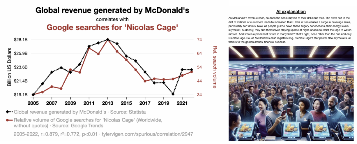
There is a well known principle in statistics that correlation does not imply causation. This means that even if two things change in a similar way, it doesn’t necessarily mean that one is causing the other. Just because two variables are related doesn’t mean one is influencing the other directly—they might be connected by something else or just coincidentally moving together. I attach my favourite example below, but you can see more funny stuff on https://tylervigen.com/spurious-correlations :

What’s next?
While all these statistics are mega interesting and informative, it’s hard to build full understanding of what’s going on here just by looking at numbers. Like, look at this correlation matrixes: we need to spend several minutes trying to elicit insights that we can use to answer our research questions, it requires too much cognitive power, concentration, and might just be boring.
But don’t worry: next week’s lecture will be about data visualisations, and we’re gonna build cool plots that tells this story for you. Stay tuned!
